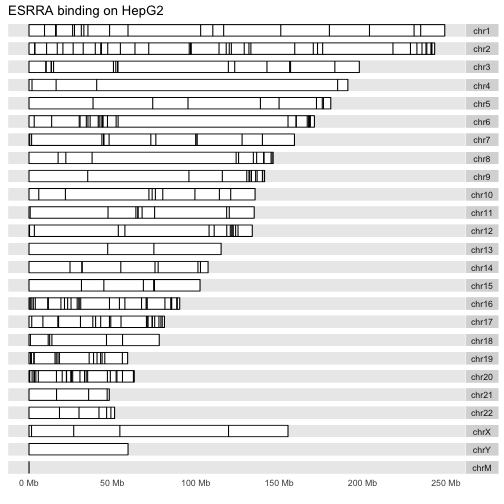
GDAS014-使用autoplot和Gviz绘图

使用ggbio包绘制染色体图

我们可以通过各种方法来绘制基因组级规模的数据。Bioiconductor中有两个这样的包,即Gvizggbio。这两个包旨在绘制基因组级数据结构的图形示意图。

ggbio 包中的 autoplot 方法用途广泛。对于GRanges实例来说,存在于每个范围中的数据都可以绘制成染色体上条带。核布图(karyogram)布局提供了全基因组的视图,不过这种图在处理染色体外序列水平方面有着重要作用。

原文如下:

The karyogram layout gives a genome-wide view, but it can be important to control the handling of extra-chromosomal sequence levels.

以下是肝细胞系的布局:

1
2
3
4
5
6
7
8
9
10
11
12
library(ERBS)
data(HepG2)
library(GenomeInfoDb) # trim all but autosomal chroms
HepG2 = keepStandardChromosomes(HepG2)
data(GM12878)
GM12878 = keepStandardChromosomes(GM12878)
library(ggbio)
autoplot(HepG2, layout="karyogram", main="ESRRA binding on HepG2")
## Scale for 'x' is already present. Adding another scale for 'x', which
## will replace the existing scale.
## Scale for 'x' is already present. Adding another scale for 'x', which
## will replace the existing scale.

plot of chunk lkd

以下是B细胞系的布局:

1
2
3
4
5
autoplot(GM12878, layout="karyogram", main="ESRRA binding on GM12878")
## Scale for 'x' is already present. Adding another scale for 'x', which
## will replace the existing scale.
## Scale for 'x' is already present. Adding another scale for 'x', which
## will replace the existing scale.

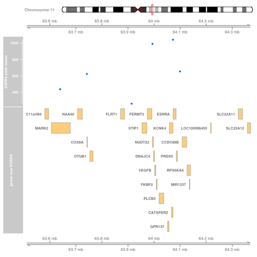
使用Gviz包绘制ESRRA结合位点与基因注释

我们通常会将观察到的数据放在基因组的参考信息中来绘制这些数据的图形。现在我们演示一下如何ESRRA结合的图形。

第一步我们先加载相关的数据、注释包与Gviz包,如下所示:
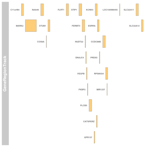
1
2
3
4
5
library(ERBS)
library(Gviz)
library(Homo.sapiens)
library(TxDb.Hsapiens.UCSC.hg19.knownGene)
txdb = TxDb.Hsapiens.UCSC.hg19.knownGene

ESRRA附近的基因

我们如何确定含有ESRRA以该基因附近的人类基因组片段呢?有几种方法,我们先从ENTREZ ID开始,如下所示:

1
2
3
4
5
6
library(Homo.sapiens)
eid = select(Homo.sapiens, keys="ESRRA", keytype="SYMBOL", columns="ENTREZID")
## 'select()' returned 1:1 mapping between keys and columns
eid
## SYMBOL ENTREZID
## 1 ESRRA 2101

现在我们获取ESRRA基因的地址,并收拾它相邻基因的地址,并绑定这些基因的符号,如下所示:

1
2
3
4
5
6
allg = genes(txdb)
esrraAddr = genes(txdb, filter=list(gene_id=2101)) # redundant...
esrraNeigh = subsetByOverlaps(allg, esrraAddr+500000)
esrraNeigh$symbol = mapIds(Homo.sapiens, keys=esrraNeigh$gene_id, keytype="ENTREZID",
column="SYMBOL")
## 'select()' returned 1:1 mapping between keys and columns

使用Gviz 包快速绘制图形,如下所示:

1
plotTracks(GeneRegionTrack(esrraNeigh, showId=TRUE))

plot of chunk lknei

此区域内的ESRRA结合峰

我们从某个样本(GM12878 EBV-transformed B-cell)获取ESRRA结合数据,以及我们目标基因附近的子集,如下所示:

1
2
3
4
5
6
7
8
9
10
11
12
13
14
15
16
17
18
19
20
21
22
data(GM12878)
sc = subsetByOverlaps(GM12878, range(esrraNeigh))
sc
## GRanges object with 6 ranges and 7 metadata columns:
## seqnames ranges strand | name score col
## <Rle> <IRanges> <Rle> | <numeric> <integer> <logical>
## [1] chr11 [64071338, 64073242] * | 3 0 <NA>
## [2] chr11 [63913452, 63914077] * | 61 0 <NA>
## [3] chr11 [63741506, 63742754] * | 210 0 <NA>
## [4] chr11 [63992515, 63994725] * | 408 0 <NA>
## [5] chr11 [64098744, 64100083] * | 1778 0 <NA>
## [6] chr11 [63639263, 63640021] * | 2248 0 <NA>
## signalValue pValue qValue peak
## <numeric> <numeric> <numeric> <integer>
## [1] 69.87 310 32 1040
## [2] 52.48 123.72 1.785156 259
## [3] 18.24 59.652 2.022276 622
## [4] 9.04 41.001 1.910095 990
## [5] 9.03 19.758 2.075721 653
## [6] 8.65 17.481 2.031517 436
## -------
## seqinfo: 93 sequences (1 circular) from hg19 genome

计算表义文字(ideogram)从而给出染色体体的信息

计算过程有点慢。

1
idxTrack = IdeogramTrack(genome="hg19", chr="chr11")

数据合并

我们从顶部开始,用表意文字来确定染色体和染色体上的区域,并且通过观察到的数据和结构信息放大这个区域,如下所示:

1
2
3
4
plotTracks(list(idxTrack, GenomeAxisTrack(),
DataTrack(sc[,7], name="ESRRA peak values"),
GeneRegionTrack(esrraNeigh, showId=TRUE,
name="genes near ESRRA"), GenomeAxisTrack()))

plot of chunk dofull

参考资料

  1. Sketching the binding landscape over chromosomes with ggbio’s karyogram layout
  2. Gviz for plotting data with genomic features